Monitoring Hybrid Rating Systems and the Role of Cyclicality

13 September 2022

13 minute read

Read our white paper below download it here.

Firms are continuing to work through the initial and ongoing PRA feedback regarding the development of Mortgage IRB PD models to meet the new regulatory requirements contained in SS 11/13 following the release of PS 13/17. However, an area that has seen less focus to date has been that of monitoring, although we are aware of recent challenges from regulators on how this will be addressed.

The monitoring of a hybrid rating system introduces new considerations to IRB monitoring, as the expectation of accuracy is that the model does not predict perfectly but does track the trend in the observed default rates to an extent. This is defined as the cyclicality of the rating system.

This deviates from most existing approaches whereby a simple comparison of actual vs expected is required for Point in Time (PiT) approaches or there is limited consideration of short-term accuracy with Through the Cycle (TtC)/long run approaches. Even with existing hybrid type approaches, often seen in IRB models for commercial lending, the focus on ‘accuracy’ and ‘cyclicality’ is not at the level anticipated for mortgages given the PRA feedback during developments.

This new requirement introduces the need to have an expectation of the movements in the observed default rate, the PD produced by the rating system and the associated drivers. This paper explores approaches and challenges with regard to assessing whether the overall modelled PD is in line with expectations and therefore focuses heavily on the cyclicality of the rating system as a key driver.

It should be noted that monitoring principles of the other key aspects – discrimination and stability is not expected to fundamentally change from current practices although there may be some additional considerations. For example, confidence intervals for risk grade default rates and continuous score vs pooled discrimination amongst others.

Overall Model Accuracy assessment

To support our thinking in the area of overall accuracy monitoring we have developed an illustrative hybrid model using publicly available information contained in the Freddie Mac Single Family Loan Level Dataset. This model was developed utilising data from 1999 to 2015 to allow a monitoring period post 2015 to be considered, simulating a real-life historical deployment. It is acknowledged that the final model is not necessarily compliant with all PRA requirements but was sufficient to explore the concept of accuracy monitoring.

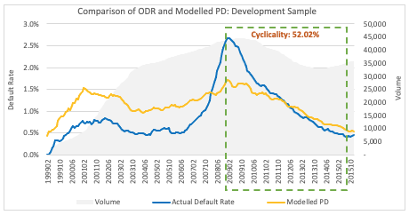
The main area of interest is understanding the level of cyclicality that the model could be expected to exhibit over the monitoring period. As is currently common practice with the ongoing hybrid model builds, during development a single view of cyclicality was defined based on a peak to ‘local trough’ observed default rate (ODR) movement (although it is understood that this view is likely to need to be expanded to consider other periods before final submission). However, as it is unlikely the monitoring period would contain a similar period, an acceptable variation in cyclicality in recent times needs to be understood.

On this basis, several options were explored to quantify the expected level of cyclicality based on the movement in the actual default rate. The aim is that, if an acceptable level of cyclicality can be understood, then this can then be used to derive the boundaries that the modelled PD should sit within based on the ODR movement. The model accuracy can then be assessed by comparing the modelled PD (from the rating system) with the ‘expected PD’ (based on the cyclicality).

As would occur with live monitoring, all parameters were developed using data within the development window and then applied to the monitoring period.

Initial Approach: Single Cyclicality based on the latest cycle (Latest Peak to Trough: Jan 2009 – August 2015)

In this approach, cyclicality is calculated based on the latest peak to trough period (in this example, Jan 2009 – Aug 2015), which produces a cyclicality measure of 52.02%.

This cyclicality is then used to create an expected PD. Two approaches are considered in the application of the single cyclicality to create an expected PD.

Approach-1a

In this approach, for each monitoring period the ‘Expected PD’ is derived from the previous monitoring period based on the movement in the observed default rate (ODR) and the quantified level of cyclicality.

As this approach always uses the Expected PD, it does not correct itself based on how the modelled PD has tracked the ODR since development. Therefore all deviation between modelled PD and ODR since development is reflected into the latest monitoring values.

Approach-1b

Alternatively, an approach could only consider more recent deviations between ODR and modelled PD. This could adjust the modelled PD of 12-month prior (instead of from deployment), based on the movement in the observed default rate (ODR) and the quantified level of cyclicality (note that alternate periods could be used but 12 months is considered reasonable for this example).

Comparsion

The two approaches each have advantages and disadvantages, dependent upon the usage. Approach 1a will continue to show deviation in the current estimates due to the historical path of the ODR vs the modelled PD regardless of the time elapsed since the occurrence. This could be seen as advantageous when compared to approach 1b as it ensures that monitoring does not have the ability to trend back to green if prior unexplained variances are not addressed, as would happen after 12 months with approach 1b. However, if an organisation is confident of its ability to remediate any genuine concerns in a timely manner, it would be assumed that any unaddressed deviation has been analysed and comfort given that it is not of concern. In this instance approach 1b would be preferable as it would consider recent deviations.

The charts below the impact of applying these methods to the theoretical monitoring period.

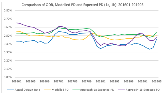
Due to the reliance of the modelled PD 12-month’s prior and the short shocks to the ODR, Approach 1b is significantly more volatile and shows a greater ‘error’ between the modelled PD. This is particularly at the start of the series, which is driven by a large fall in the modelled PD over the prior 12-months and also from mid-2018 where there is a large increase in the expected PD. The impact of the movement in the expected PD from 12m prior be seen when the drivers are isolated.

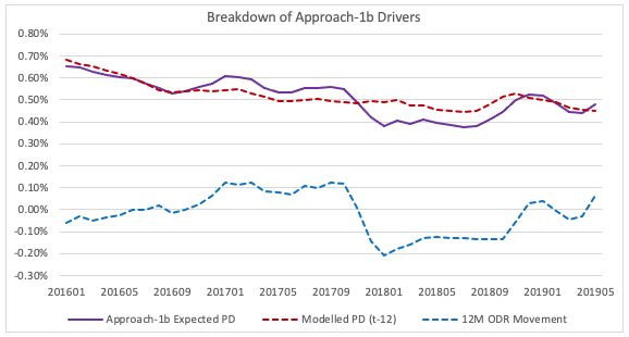
As can be seen is certain periods, e.g., Q1-Q3 2016, the movement in expected PD is heavily driven by the previous movements in the modelled PD (at t-12) rather than the shift in ODR. However, in periods of large ODR movement e.g., Q4 2017, it does react well to the movement in ODR. This is different to approach 1a, which has a much smaller reaction to the change.

Tolerances: Lower and upper bounds for cyclicality based on the observed trend during development

The initial approaches considered each give a singular view of the expected PD. However, for monitoring purposes there needs to be a level of tolerance as the modelled PD will likely never align exactly with expectations.

To consider the assessment of tolerances, the development data is used to calculate cyclicality for 12-months interval (based on the latest cycle, i.e., latest peak to trough 200901-201508) and capped/floored between -100% and +100%. Further, to get rid of the negative cyclicality, the trend is analysed only for cases with Cyclicality greater than 0% (omitted points are shown in red in the chart below).

The quantified level of cyclicality for each period can be compared to the movement in ODR over the same period. This is an important consideration as the monitoring period may have significantly different ODR movements to that seen over development window.

From the scatter plot below, it can be observed that cyclicality is not static, but does follow a well-defined trend. It is generally observed that it is higher and very volatile when the magnitude of default rate change is lower, and lower and less volatile when the magnitude of default rate change is significantly higher.

Two clusters have been identified from the scatter plot, based on the mean and standard deviation of cyclicality within the clusters. It should be noted that alternate approaches are available whereby regression lines are fitted through the data points (or log transformed points) and upper lower bounds estimated from this. However, for simplicity and explain ability we have taken a more basic approach here.

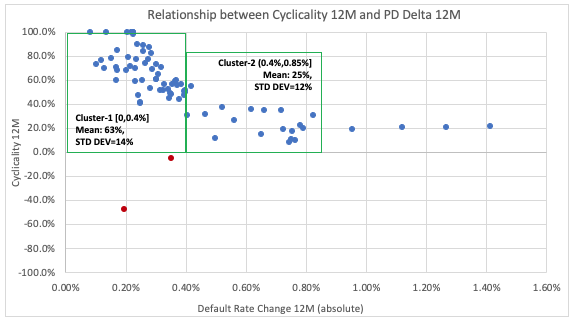
Using these clusters upper and lower bounds of cyclicality have been assessed using 2-standard deviations to represent a c95% confidence interval.

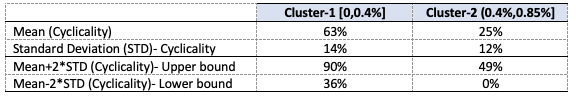
In this example we arrive at a 0% lower bound for cluster 2, which would need to be assessed in more detail and likely overridden in a full monitoring development.

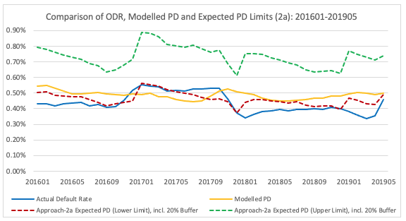
As with Approach 1, using these lower and upper bound of cyclicality, an “expected PD range” can be derived. The modelled PD will be assessed against this “range” during the ongoing monitoring of the model. In this example no RAG threshold has been set however, this approach can be used with varying confidence intervals to set green, amber, and red tolerances.

Approach-2a – inclusion of tolerances to Approach 1a

As an extension to Approach 1a, this approach considers the change in lower/upper limits for the ‘Expected PD’ from 12-month prior- would depend on the movement in the observed default rate (ODR) and the quantified level of cyclicality.

Additionally, it was considered that a near flat ODR should not necessarily be expected to result in a near flat modelled PD (as would occur with the underlying approach) due to general inherent model volatility. Therefore, it is proposed that a buffer needs to be considered in the lower and upper limits of the expected PD to arrive at a reasonable range. Otherwise, if there is no or very little change in the observed default rate between t and t-12, then both the Lower and Upper limits of the expected PD will be almost the same with little tolerance applied to the expected PD. Results with no buffer options are presented in Appendix-D.

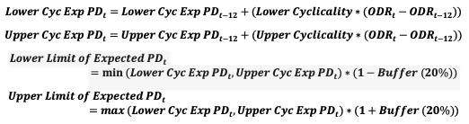
Note, Lower and Upper Cyclicality will be applied based on the magnitude in default rate change. If Delta<=0.4%, then lower and Upper limit of Cluster-1 will be used, else for Cluster-2.

Approach-2b – inclusion of tolerances to Approach 1b

As an extension to Approach 1b, expected PD limits are derived in similar fashion as 2a, but adjusting the Modelled PD instead of the expected PD of 12-month prior.

As an extension to Approach 1b, expected PD limits are derived in similar fashion as 2a

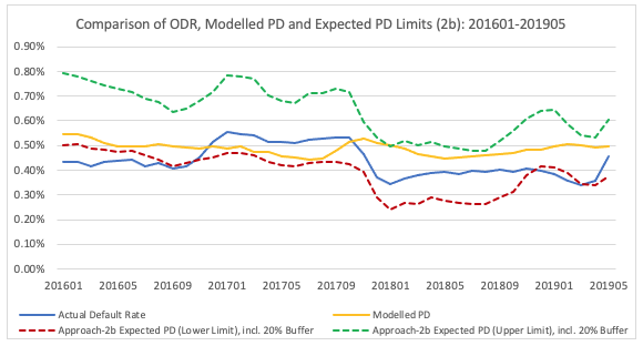
As would be expected, similar to Approach-1, in periods of large ODR movement (for example Q4 2017), the approach-2b reacts more compared to Approach-2a. Approach 2a has a relatively smaller reaction to the change due to the fall in ODR being partially offset by a rise in ODR during Q4 2016.

Further Analysis: Relationship between Cyclicality and Default rate change from the latest Peak (February 2009)

Another approach considered when assessing the expected level of cyclicality was to set the latest peak (February 2009) as the anchor point and derive the relationship between cyclicality and default rate change of these observations. This approach is more aligned to the PRA guidance on the assessment of cyclicality.

As with the other approaches a strong linear relationship can be seen between the cyclicality and absolute default rate change from the latest peak.

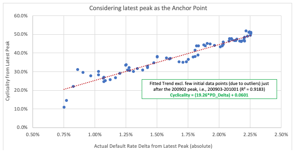
However, although we are getting a strong linear relationship between PD Delta and Cyclicality, the trend is opposite compared to that seen in other analysis (present in Appendix-C), where there isn’t the anchoring of one of the points. In other options seen earlier, a negative relationship is observed between cyclicality and the magnitude of PD Delta. But, in this approach the cyclicality reduces with a decrease in magnitude of PD Delta.

However, upon investigation the reason for this difference in trend is due to the behaviour over differing time intervals within the period, rather than a fundamental reversal of previous findings.

As the default rate is falling over the entirety of the period of interest, the data points relating to the larger deltas in ODR are, by definition, where t is further away from t-1 ie. t is later in the period, as shown in the left-hand chart below. However, the movement (slope) of the ODR delta begins to decrease in the later months, and this coincides with the ODR and model PD moving in greater sync, as can be seen in the right-hand chart ie. the cyclicality begins to increase as the short term deltas reduce, as was observed in the earlier analysis. This results in the overall cyclicality increasing for the data points where it is in the later months and the marginal deltas are low but the cumulative delta from peak is still increasing, albeit at a lower rate.

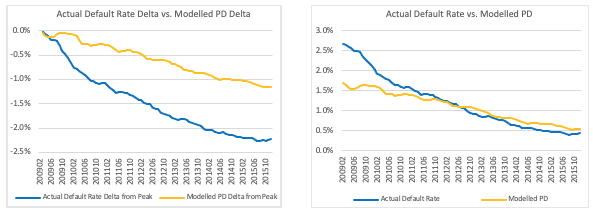
Therefore, this apparent change in relationship between cyclicality and ODR delta can be explained as being due to the time period they are taken over and change in the cyclicality observed over differing rates of ODR change.

It does however raise a consideration which is with regards to the impact of time interval on the level of cyclicality. Some initial analysis has been undertaken to assess the results on both a 12m and 24m period (contained in Appendix-C) and it does show that the 24m interval is more stable and delivers higher quantified cyclicality levels for smaller ODR deltas.

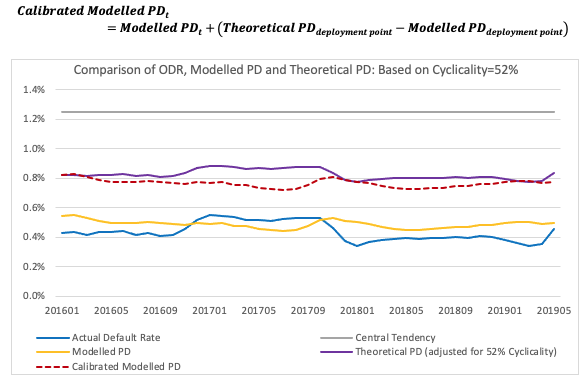
Theoretical PD by applying cyclicality to the difference between Observed Default Rate and the Central Tendency

Another approach tested is based on the ‘Theoretical PD’, by applying the cyclicality to the difference between the observed default rate and the central tendency, adding that value back onto the central tendency, and comparing that to the modelled PD.

Central Tendency (1.24%) is the long run average PD, i.e., the time-weighted avergage of actual default rate calculated over the economic cycle (i.e., trough to trough period: 200606-201509).

As can be seen in the chart below, the modelled PD is well below the theoretical PD throughout the monitoring period. This is because the actual default rate has reduced significantly in the recent period and is very low compared to the central tendency (1.24%) calculated over the economic cycle (200606-201509). Even at the point of deployment (i.e., the first monitoring month 201601), a big difference can be observed between the theoretical PD and the modelled PD. This has been raised as a concern previously by the PRA and also makes any attempt to apply go forward monitoring using this approach very difficult given the constant large deviation. One simple solution (for the purposes of this example) could be to derive an adjustment factor at the point of deployment and use that factor to calibrate the modelled PD for the monitoring purposes.

Once calibrated, this approach delivers very similar results to Approach 1a outlined earlier. This is intuitive as both ignore any prior movements in the modelled PD and embed all movements from and deviations from the point of deployment.

Conclusion

As outlined above, this is a focussed investigation of the impact that cyclicality has on the monitoring of hybrid PD and tries to outline where thinking needs to go in order to address the complexity of the challenges to be faced. The consideration regarding the variability of cyclicality and how this is impacted by factors such as ODR delta and time period have been the focus of PRA discussions but not necessarily with regards to how this impacts monitoring. As with any monitoring framework, the proposed solution will need to ensure that it can provide timely insights into the deterioration of the rating system but also protect against unnecessary responses to simple variation and volatility. It is felt that the analysis presented here provides firms with starting guidance as to approaches that will be fulfil this need.

It is acknowledged that the approaches detailed here could also be addressed by monitoring the cyclicality directly rather than its impact on a ‘expected PD’. However, it is felt that PD accuracy is a known measure in monitoring and that the analysis presented would form part of a wider investigation that may result in the adjustment to the monitoring ODR, based on observed changes in ODR outside of the cycle such as acquisition strategy or collections practices. If these adjustments were to take place it is felt that it would be easier for business understanding as to the impact on the ‘accuracy’ of the model.

Additionally, to reiterate, it should not be forgotten that a full monitoring solution will require further metrics, both standard and new, alongside the overall ‘accuracy’ of the rating system. These other considerations should also support with the consideration of the accuracy performance and will likely include (but not be limited to) understanding of the ODR performance with risk grades, overall discrimination of the model and portfolio ODR performance compared to the industry.

Appendix-A: Cyclicality trend based on the Overlap and Non-Overlap data points

Due to the very strong relationships seen in the analysis presented, upon review concern was raised with regards to whether the large clustering was due to overlapping data periods containing very similar cyclicality and ODR deltas. Hence, analysis was undertaken to understand if these trends changes drastically if it is derived based on overlapping or non-overlapping data points. Whilst the relationship is not as strong, as would be expected due to the independence of the points and lower volumes, the overall trend is still aligned to prior results.

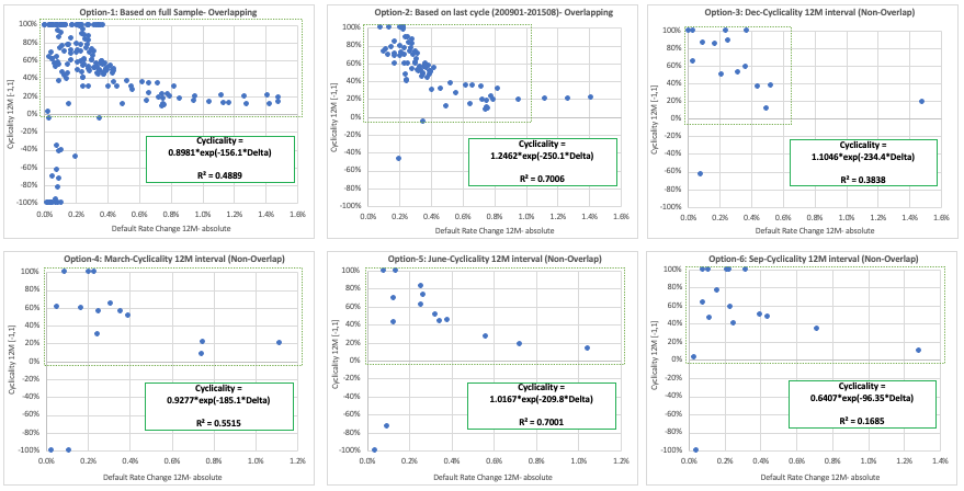
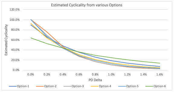
The similarity of the trend is further evidenced when, based on these scatter plots (shown above), exponential trend lines are fitted.

As can be observed in the chart below, the estimated cyclicality is very similar across all these options except Option-6 (i.e., based on the September trend). It can be noted that for option-6, the R-square is also very low (17%) compared to the other options.

Appendix-B: Cyclicality trend by Low, Medium & High buckets

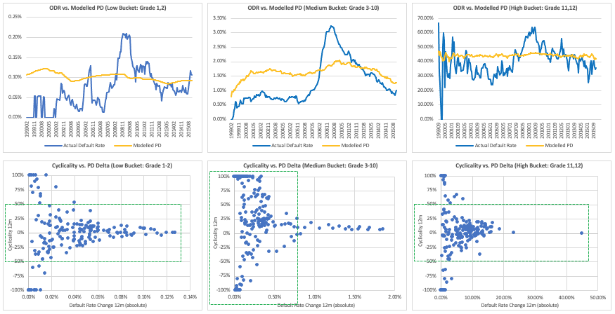
As part of the overall monitoring process, it will be necessary to consider more granular views and in particular underlying risk levels. Therefore, as an initial investigation, analysis was undertaken to understand if the cyclicality trend differs by aggregated risk buckets (the buckets are defined based on the PD grades). It is observed that the cyclicality is relatively low and less volatile for the Low (Grade=1,2) and High (Grade=11,12) PD buckets compared to the Medium (Grade=3 to 10) bucket. This analysis, alongside individual risk grade default rates, can be used for more detailed monitoring of the rating system.

Appendix C: Relationship between Cyclicality over 12M and 24M intervals

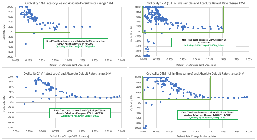
Consideration was given to the assessment of cyclicality over both 12m (as per the original assessment) and 24m. Similar trends have been observed and the higher default rates indicate a similar overall level of cyclicality (circa 20%), however the 24m period does give a higher level of stability, as evidenced by the more stable R-square. Additionally, for lower ODR deltas, the 24m period does on average give a higher level of cyclicality, for example for ODR deltas less than 0.5% the average cyclicality for 24m period is 81% compared to 52% based on the 12m period (considering full in-time sample).

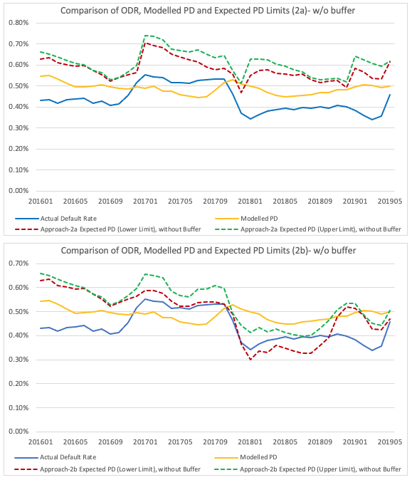
Appendix D: Results for Approach-2 with no buffer options

In Approach-2 (as discussed previously), a buffer is considered in the lower and upper limit of the expected PD to arrive at a reasonable range. Otherwise, if there is no or very little change in the observed default rate between t and t-12, then both the Lower and Upper limits of the expected PD will be almost the same with little tolerance applied to the expected PD. Results for both Approach-2a and 2b with no-buffer options are presented below. As can be seen, the lower and upper limits are almost the same in 2016Q1-Q4, as the change in the observed default rate compared to 12m prior is very low.